Alzheimer's Disease Detection

This project was also my master's thesis, where I used a support vector machine (SVM) to identify whether Alzheimer's Disease (AD) was present in brain magnetic resonance imaging (MRI) data and then implemented a convolutional neural network (CNN) to then measure the severity of any identified Alzheimer's Disease. The project also implements several sampling techniques that are collectively referred to as Synthetic Minority Oversampling Techniques (SMOTE).

Data Overview

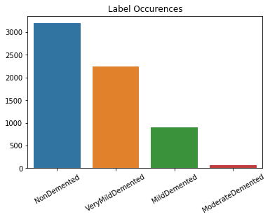
The data consisted for 6,400 T1-Weighted MRI brain scan images of patients with and without AD. The images were gathered from multiple online sources, the primary of which was the Open Access Series of Imaging Studies (OASIS). The images were labeled via professional evaluation as: non-demented, very mild demented, mild demented, and moderate demented.

Of the two meta-categories (demented and non-demented), there was an even split between the data, with 3,200 images in each category (Fig. 2). However, this resulted in the sub-labels, measuring the severity of the condition, being heavily skewed towards the non-demented category (Fig. 3). This is what ultimately led to the implementation of the SVM, to completely eliminate the non-demented label from the severity classification and SMOTE to more evenly distribute labels.

SMOTE

Originally proposed in 2002 by Chawla et. al., SMOTE's goal is to create more robust, reliable datasets by identifying under-sampled classes and creating "synthetic" samples to supplement these classes. It does this by finding the n nearest neighbor samples to one of the under-represented samples and then creating a new sample by using the mean of the neighbors, adjusted by random noise. The success of Chawla et. al.'s original research and the continued popularity of the technique makes it a strong candidate for sampling issues like the one above.

Models

SVM Binary Classification

This model was built off of scikit-learn's LinearSVC model and using the hinge loss function. After training, the model was exceptionally adept at identifying MRI images with AD and those without. It was so accurate, in fact, that further analysis was performed on the data, to ensure there were no hidden artifacts that were making prediction easier. None were found.

As seen in figure 4, only 30 of the 2,240 test samples were misclassified in the final version of training. Furthermore, after examining the errors, the 11 false negatives were all "very mild demented" samples, that were predicted to be non-demented. This suggests that the early stages of AD are more difficult to identify than later stages. Even so, only 30/2,240 misclassifications is a very acceptable margin of error for this and most any model.

CNN Multi-Class Classification

Implementing the CNN (which was built using Keras and TensorFlow) was more complex than the SVM, as this is where SMOTE was also implemented. When using SMOTE, the how is obviously very important, but the when is equally as important. Nick Becker, at NVIDIA, talks about this and how important it is to implement SMOTE on only the training data. Even though the synthetic data is technically completely new, the sub-features of the data are not and therefore could lead to a contaminated training set. With this in mind, the CNN pipeline was:

1. Ingest the data.
2. Perform the general data cleaning/preparation techniques.
3. Split the data into training and test sets.
4. Apply SMOTE to the training set, putting the synthetic samples into the training set.
5. Perform any training set specific data cleaning/preparation techniques, such as scaling and normalization sets (it is important to do this after SMOTE, as the synthetic samples will be scaled and normalized as well).
6. Complete the training/testing process.

Another important consideration with SMOTE is that it needs to be replicable. This is because the training set for any given iteration needs to be available for future testing and validation. Luckily, this can be done relatively easily by implementing seeding into the process and with thorough testing.

The design of the CNN layers was based on core principles of CNNs laid out by Yann LeCun in his 1995 paper. The main ideas are: several matching convolutional layers, followed by a max pooling and dropout layers, to prevent overfitting. Then repeating this pattern multiple times; in the case of this project, it was repeated three times. Finally, the model ends with a flattening layer and two dense layers. Each convolutional layer uses ReLu activation and the final dense layer uses softmax activation, the standard for multi-class classification.

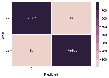
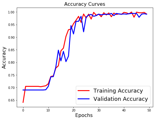
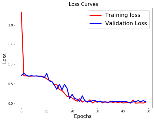
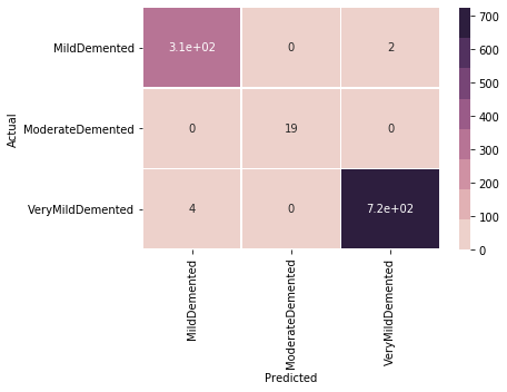
The final model was able to achieve an accuracy of 0.99 (Fig. 5), which is very good. It is important to note that this is not the only metric that was considered, but all others showed similar levels of positivity. The confusion matrix (Fig. 7) shows that the model performed very well overall. In particular, it is encouraging that the sparsest feature set (ModerateDemented) was correctly labeled 100% of the time, which suggests that the most likely form of bias was avoided. The only other pattern that can be gleaned from the matrix is that all errors were a result of VeryMildDemented and MildDemented being confused. This is consistent with the general logic that the lines may blur between the two lower categories and professionals might draw different lines between them. Regardless, the sheer accuracy of the model is encouraging.

Conclusion

At the end of the day, the ultimate goal of a machine learning project is to create a strong model, which I can safely say was accomplished. But looking beyond that, this project was a good opportunity to explore a variety of techniques and infrastructure within data science. SMOTE is a very powerful tool, in the right scenario, and it was good to have a chance to implement in a realistic way. On top of that, it is often overlooked how important the machine learning pipeline itself is to a project. In particular for this project, a pipeline that utilizes two different models to enhance the performance of each other, is a very powerful approach that is often ignored unless discussing Generative Adversarial Networks (GANs).