Audio MNIST Deep Learning

Using the audio MNIST dataset, created by Becker et al. for their paper "Interpreting and Explaining Deep Neural Networks for Classification of Audio Signals", I perform deep learning, using a PyTorch Neural Network, to accurately identify numbers being spoken.

Data

The data consists of 30,000 audio samples stored in .wav files. These samples are evenly distributed between the numbers 0-9 and between 60 speakers. Each speaker speaks the same number for the same number of iterations as every other speaker.

Analysis

The process for the analysis itself can be found in the Jupyter notebook data_analysis.ipynb.

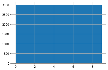
The Labels

The labels were examined to confirm their distribution and, as seen in the graph below, all labels had the exact same number of samples (3,000).

Sample Rates

For audio modeling, sample rates are important because it lets you know how much data you are getting in one second of audio, much like resolution in images. When the data is prepared for modeling, ensuring each clip has the same sample rate is important to get accurate results.

Examining the sample rates of each sample within this dataset reveals that they all have the same sample rate of 48,000.

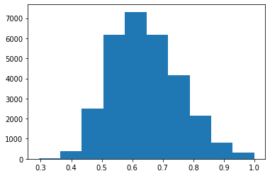
Sample Lengths

Much like image modeling, all audio samples will need to be the same length to get passed into the model.

Looking at the histogram below, the lengths are normally distributed, no less than 0.3 seconds, and no greater than 1 second. The shorter lengths will need to be padded by some method to allow modeling.

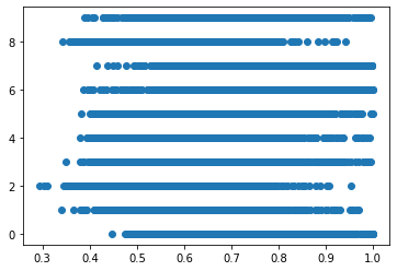
In addition to examining the distribution, it is important to also understand how each individual label's sample lengths are distributed, to ensure the model does not overfit based on clip length.

The scatter plot below shows that, while some numbers have higher floors and others lower ceilings, the majority of clip lengths are gathered around the mean of clip lengths, which is good for modeling. To be more specific, no label has a mean clip length less than 0.55 seconds or greater than 0.73 seconds.

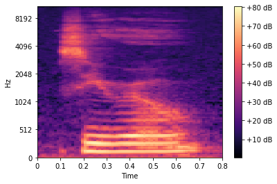
Mel Spectrogram

Before moving to data preparation, it is good to understand how the data will look prior to our model. In the case of audio data, instead of feeding a model raw samples, it has been shown to be more effective to feed neural networks spectrograms--images of the audio--to process how you would normally model images.

Mel Spectrograms in particular are effective for audio monitoring as they apply a Fourier Transformation and then scale the audio to fit within the more visually usable Mel Scale.

There are many libraries, including some built into PyTorch, Librosa, or scikit-learn, that can create Mel Spectrograms. The below example was made using Librosa, but PyTorch will be used for the actual modeling, as that makes a cleaner pipeline.

Data Prep

To prepare the data, the audio samples are stored in a custom AudioData class, which is built on PyTorch's Dataset class. Once in AudioData, cleaning/processing functions are called from the custom class AudioUtil (both AudioData and AudioUtil can be found in utils.py).

Once the file is read in, five cleaning steps occur, based on the results of analysis, in addition to best practices for audio data preparation:

1. Resample: The sample is passed through AudioUtil.resample() using torchaudio's Resample function to adjust the sample's sample rate to the default sample rate identified in analysis (48,000).
2. Rechannel: Much like the variance of images and their different color schemes (RGB, GRB, etc.), audio can be created on one or two channels. The model will expect two channels, so all one channel samples are converted to two channel.
3. Pad/Truncate: This sets all samples to a default length (in this case 1000ms or one second), using white noise to pad.
4. Mel Spectrogram: The sample is then converted to a Mel Spectrogram using PyTorch's Mel_Spectrogram() function.
5. Random Masking: Random frequencies and periods of time are blocked out in each spectrogram, creating additional noise to prevent overfitting and improve generality.

Modeling

The model itself can be found in models.py. It has four layers and mostly follows standard CNN structure best practices. Each layer uses ReLU activation and a kaiming initialization, which will take into account the ReLU's non-linearity. At the end, the model passes the inputs through an AdaptiveAvgPool2d() and then converts the output to linear, with 10 different options.

The process of training and testing the data can be found in classify.py. Here the audio files are gathered, the AudioData class is initialized, the data is split, trained, and tested.

During training, TensorBoard was used to monitor the progress of training and the performance of the model. A writer was initialized in classify.py, then functions were called from the TensorBoard class in utils.py to write results to TensorBoard.

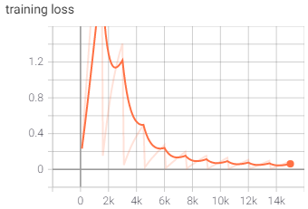
Each of the versions of the model below had 10 epochs, since, as you will see, more training after 10 was not necessary.

Results

There were three full iterations of the model, with smaller iterations during each major phase. This will just review the final results of each iteration. The majority of work between phases revolved around improving the data quality, as the model structure was plenty effective from the outset, so the main goal was avoiding overfitting and erroneous labeling.

Version 1

The first version of the model set 1500ms (or 1.5 seconds) as its default clip length and padded each sample with white space to reach that length. Then all the other transformations were performed and the data was passed into the CNN.

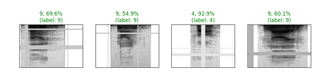
Referencing the picture below, which takes place in epoch 4 and is a sample of 4 validations, the model is already doing an impressively strong job at identifying each number correctly, hovering around 0.82 accuracy.

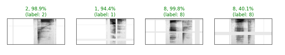
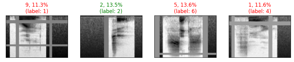
As the training progresses and the model becomes even more accurate, you can still identify some areas which give the model some difficulty. In particular, you can see in the image below, that samples that have large portions of the beginning of their clip masked, have lower accuracy than those without that masking.

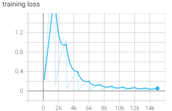
When training was complete, the model had a final Loss of 0.06 and a testing accuracy of 0.98.

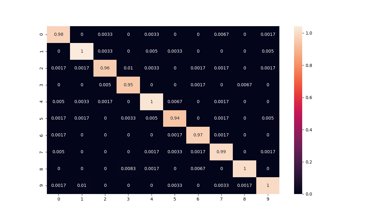
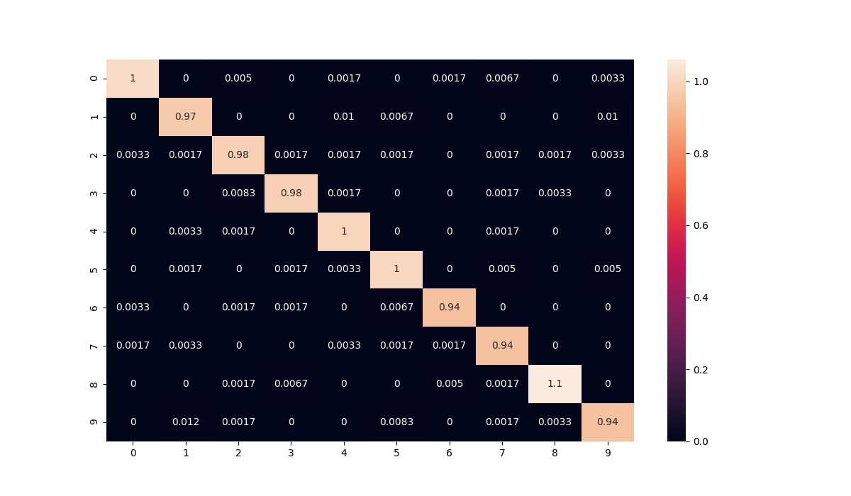
Examining the confusion matrix of the test dataset, it is also clear that no single label is more or less accurate than the others, adding credence to the hope that the errors are random and not caused by a specific set of labels.

Version 2

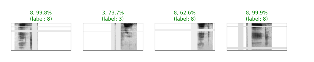
One concern coming out of iteration 1 was that the padding is too large, somehow causing the model to overfit and inflate the accuracy. To ensure this wouldn't happen, iteration 2 was identical in all aspects to 1, but the default clip length was reduced to 1000ms.

You can see clearly in the sample images that the padding is noticeably reduced and the training progression suggested some changes as well. The model stayed at lower accuracies and high losses longer than iteration 1, but by the time it finished training it had both improved on accuracy and loss.

After being trained and tested, the model had a final Loss of 0.04 and a testing accuracy of 0.99.

Version 3

Feeling more confident about the model, there was one key thing I wanted to implement for a final iteration: white noise. Instead of white padding on either edge, I wanted to introduce truly random white noise so that the model could be more comfortable with background noise. To do this, I removed the white padding and replaced it with random padding in the frequency range of the current sample.

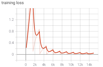
With the white noise implemented (see below), the model had a much tougher time initially, doing poorly until about epoch 4. Once there it began to improve rapidly and achieved the same loss and accuracy of iteration 1.

After being trained and tested, the model had a final Loss of 0.05 and a testing accuracy of 0.98.

To confirm consistency from iteration 1, the confusion matrix is examined again with similar results. (The confusion matrices of all other iterations and k-folds can be found in figures)

K-fold Cross Validation

Feeling very confident in this third iteration, one more best practice I wanted to implement was K-fold cross validation.

Using scikit-learn's KFold class, I performed 5-fold cross validation on the samples, using the same model and data prep process as iteration 3.

Results:

• Loss: 0.04; Acc: 0.99
• Loss: 0.03; Acc: 0.99
• Loss: 0.04; Acc: 0.99
• Loss: 0.03; Acc: 0.99
• Loss: 0.04; Acc: 0.99

With cross validation producing very similar results to the rest of my training iterations, I feel comfortable saying that this is a strong model for classifying spoken numbers.

Live Classification

To show the model in action, I have included live_classify.py, a script that allows you to live record your own voice and classify the numbers you say. To use this script, simply run it in terminal with python live_classify.py, wait for "Ready to record..." to appear, then press R to record for 1.5 seconds, after which the model will classify what you said. Press Q to quit.

Note: The Python library sounddevice may not work on some OS's or with certain microphones, so some tweaking may be required before you can run the script in its entirety.

Note 2: Since the saved models and data are not in this repo, wrangling and training will need to be done first prior to using this script.

Next Steps

Just because I am comfortable with iteration 3, does not mean there is no work left to be done.

More Data

30,000 well-distributed samples is a great starting point for this model, but there are some ways I would like to see it improved and built upon:

• A higher variety of speakers: This dataset had 60 different speakers, but slightly more than half of them had German accents, with the rest having other varieties of European and African accents. It would be nice to incorporate additional data with American and Asian accents.
• A higher variety of circumstance: All recordings for this dataset were recorded professionally, with minimal background noise or blank noise on either side of the number. A future iteration with more variety in the circumstances of the speaker (with background conversations, with background music, yelling, whispering, etc.) would continue efforts to limit overfitting.

More Prepping

The padding, white noise, and masking done for preparing this data is a strong starting point to generalize the model, but further steps can be taken, such as more aggressive masking, to continue ensuring the model's generalizability.